RE: The anatomy of my pet brain
ListfitnessSet= newArrayList<>(); fitnessSet.add(this.net .add(newSqLossLayer(), this.feedback, this.net.getInput().get(0)) .add(newAvgMetaLayer()).getHead()); fitnessSet.add(this.net.add(newSparse01MetaLayer(), this.center) .add(newSumReducerLayer()) .add(newLinearActivationLayer().setWeight(.1).freeze()).getHead()); fitnessSet.add(this.net.add(newSumInputsLayer(), weightNormalizationList.stream().map(x->net .add(newWeightExtractor(0, x), newDAGNode[] {}) .add(newSqActivationLayer()) .add(newSumReducerLayer()).getHead()).toArray(i->newDAGNode[i])) .add(newLinearActivationLayer().setWeight(0.001).freeze()) .getHead()); this.net.add(newVerboseWrapper(“sums”, newSumInputsLayer()), fitnessSet.toArray(newDAGNode[] {}));
## Trainer Methods
Although I have played with an experimented on variations of the learning algorithms, my first published version is sufficient with a first-order [gradient descent](https://github.com/acharneski/mindseye/blob/blog20151018/src/main/java/com/simiacryptus/mindseye/training/GradientDescentTrainer.java) procedure with a simple [adaptive rate](https://github.com/acharneski/mindseye/blob/blog20151018/src/main/java/com/simiacryptus/mindseye/training/DynamicRateTrainer.java). Alternate methods such as [L-BFGS](https://en.wikipedia.org/wiki/Limited-memory_BFGS) and [PSO](https://en.wikipedia.org/wiki/Particle_swarm_optimization) are planned for the future. Outside these methods (implemented and not), there are a variety of methods to select training sets to optimize learning, putting the “stochastic” in stochastic gradient descent. This method is used, implicitly, by several test examples.
# Results
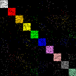
## Classification Regions
To help visualize and explore the behavior of these systems at low dimensions, I've created a [suite of test categorization problems](https://github.com/acharneski/mindseye/blob/blog20151018/src/test/java/com/simiacryptus/mindseye/test/demo/shapes/SoftmaxTests2.java#L16). This uses a randomly set of population points in 2d space drawn from a variety of patterns. Some patterns are easy for a simple network to classify, and others are nearly impossible (for simple networks):
ClassificationResultMetrics [error=0.13045791649812016, accuracy=1.0, classificationMatrix=[ [ 100.0,0.0 ],[ 0.0,100.0 ] ]] TrainingContext [evaluations=Counter [value=698.0], calibrations=Counter [value=0.0], overallTimer=Timer [value=0.0], mutations=Counter [value=0.0], gradientSteps=Counter [value=162.0], terminalErr=0.01]ClassificationResultMetrics [error=0.18390882304814632, accuracy=1.0, classificationMatrix=[ [ 100.0,0.0 ],[ 0.0,100.0 ] ]] TrainingContext [evaluations=Counter [value=100558.0], calibrations=Counter [value=0.0], overallTimer=Timer [value=0.0], mutations=Counter [value=0.0], gradientSteps=Counter [value=23206.0], terminalErr=0.01]ClassificationResultMetrics [error=1.0292766269432674, accuracy=0.995, classificationMatrix=[ [ 100.0,0.0 ],[ 1.0,99.0 ] ]] TrainingContext [evaluations=Counter [value=102551.0], calibrations=Counter [value=0.0], overallTimer=Timer [value=0.0], mutations=Counter [value=0.0], gradientSteps=Counter [value=23665.0], terminalErr=0.01]ClassificationResultMetrics [error=6.799908397558712, accuracy=0.615, classificationMatrix=[ [ 61.0,39.0 ],[ 38.0,62.0 ] ]] TrainingContext [evaluations=Counter [value=17300.0], calibrations=Counter [value=0.0], overallTimer=Timer [value=0.0], mutations=Counter [value=0.0], gradientSteps=Counter [value=3984.0], terminalErr=0.01]ClassificationResultMetrics [error=0.30472166219228297, accuracy=1.0, classificationMatrix=[ [ 100.0,0.0 ],[ 0.0,100.0 ] ]] TrainingContext [evaluations=Counter [value=539.0], calibrations=Counter [value=0.0], overallTimer=Timer [value=0.0], mutations=Counter [value=0.0], gradientSteps=Counter [value=125.0], terminalErr=0.01]ClassificationResultMetrics [error=0.12145764920083349, accuracy=1.0, classificationMatrix=[ [ 100.0,0.0 ],[ 0.0,100.0 ] ]] TrainingContext [evaluations=Counter [value=201.0], calibrations=Counter [value=0.0], overallTimer=Timer [value=0.0], mutations=Counter [value=0.0], gradientSteps=Counter [value=47.0], terminalErr=0.01]ClassificationResultMetrics [error=0.5919904265308571, accuracy=1.0, classificationMatrix=[ [ 100.0,0.0 ],[ 0.0,100.0 ] ]] TrainingContext [evaluations=Counter [value=20709.0], calibrations=Counter [value=0.0], overallTimer=Timer [value=0.0], mutations=Counter [value=0.0], gradientSteps=Counter [value=4779.0], terminalErr=0.01]ClassificationResultMetrics [error=0.13615430754693006, accuracy=1.0, classificationMatrix=[ [ 100.0,0.0 ],[ 0.0,100.0 ] ]] TrainingContext [evaluations=Counter [value=22.0], calibrations=Counter [value=0.0], overallTimer=Timer [value=0.0], mutations=Counter [value=0.0], gradientSteps=Counter [value=6.0], terminalErr=0.01]
## MNIST Classification
Since my main target for this project has been 2d image processing, the [MNIST](http://yann.lecun.com/exdb/mnist/) dataset is a prominent test problem. One basic step is to carry out simple supervised classification of the digits, which [our network](https://github.com/acharneski/mindseye/blob/blog20151018/src/test/java/com/simiacryptus/mindseye/test/regression/MNISTClassificationTest.java#L131) demonstrates with about a 90% success rate, which is standard for a simple logistic regression. It can train against the unsampled training set at about 250MCUPS and achieves 90% in about 2 minutes.
Here is the categorization matrix plot that is output at the end:

## MNIST Sparse Autoregression
Another experiment is [my reproduction](https://github.com/acharneski/mindseye/blob/blog20151018/src/test/java/com/simiacryptus/mindseye/test/demo/mnist/MNISTAutoencoderTests2.java#L105) of the sparse autoencoder detailed on the [standford deeplearning wiki](http://deeplearning.stanford.edu/wiki/index.php/Exercise:Sparse_Autoencoder). The network specification is the example above for a “more complex” DAGNetwork layout. The test will output a report with example images resulting from the full-feed-forward evaluation of the network (i.e. the feed-forward reconstruction) after each macro-iteration of training. Here is an example sequence a few minutes into a test run:
TEST TEST TEST TEST TEST TEST TEST TEST TEST TEST TEST TEST TEST TEST TEST TEST TEST TEST TEST TEST TEST TEST TEST TEST TEST TEST TEST TEST TEST TEST TEST TEST TEST TEST TEST TEST TEST TEST TEST TEST TEST TEST TEST TEST TEST TEST TEST TEST TEST TEST TEST TEST TEST TEST TEST TEST TEST TEST TEST TEST TEST TEST TEST TEST TEST TEST TEST TEST TEST TEST TEST TEST TEST TEST TEST TEST TEST TEST TEST TEST TEST TEST TEST TEST TEST TEST TEST TEST TEST TEST TEST TEST TEST TEST TEST TEST TEST TEST TEST TEST
Aparapi, OpenCL, JBLAS, and numerical performance
It was surprising to me that something as simple as matrix multiplication could have such nuanced performance considerations. You'd usually think of it as an O(n^2) operation, end of story. But after leveraging cpu instructions, cpu/memory cache levels, specialized hardware and native libraries, you end up getting an operation that is order(s) of magnitude faster, even if it scales the same way!
Comparing the results quantitatively is beyond the scope of this article, but I have experimented with [several variations](https://github.com/acharneski/mindseye/tree/blog20151018/src/main/java/com/simiacryptus/mindseye/net/dev) of the matrix multiplication “synapse” layer:
1. Simple, tight java loop – Performed actually pretty well, only about half as fast as JBLAS
1. JBLAS – Performed the best, uses native code.
1. Aparapi – Tested a fairly naïve kernel for matrix multiplication – Was about 50% slower than pure java, but I strongly suspect this can be improved.
(All computations are done using doubles.)
## Deconvolution
Another interesting use case for this library is image reconstruction from lossy operations such as linear motion blur. I detailed some results in this area in my previous post.
# Plans for the future
I wrote this library because I wish to experiment with these methods and compare my results with others', hopefully improving the state of the art. This post just details my experience progressing towards that end. Research ideas I have to follow up with this include:
* Alternate training methods – Many other methods – both documented in literature and floating in my head – could be used to optimize the parameters of the system.
* Additional components – I am particularly interested in structures that unify concepts such as GMM, PCA, Kernel/RBF, tree/forest, and ensemble models with neural networks.
* Aparapi optimizations and more exploration of CNNs – A large inspiration for this project has been Google's recent publications on neural network image recognition and reconstruction - I would like to continue following that line of research.
* Integration with Spark – The ability to train against larger data sets using a cluster of machines could open up interesting new lines of research, or at least could be worth writing about.
* Rewrite in scala - Many scala language features such as operator overloading, traits, and implicits could make this library much... better...er.
* Numerical/Signal Basis Transforms - Convolutional networks can be efficient to train in the fourier domain. Likewise, there can be advantages to expressing neural signals using integers or in a logarithmic basis. (Generally the advantages of such exotic approaches are gains in computational efficiency.)
More soon, I hope!