Autoencoders and Interactive Research Notebooks

Further research and development with MindsEye has produced two new features I would like to discuss today. The first is a working demonstration of a stacked sparse denoising image autoencoder, which is a fundamental tool in any deep learning toolkit. Second, I will introduce a useful tool for producing both static and interactive scientific reports, which I use to produce many of my demonstrations and conduct much of my research.

Autoencoders are one of the fundamental components of deep learning, particularly with images, and performing unsupervised learning by extracting features from data. How they work can be understood in several ways, but basically they learn how to encode the image as compressed data. Unlike a zip file or a jpg however, this compressed data itself has structure and value (see also: manifold learning). Another interesting feature is that they are recursive - applying this process on an encoded dataset will result in further structure discovery and further compression. This compressed form can in turn also be trained to remove more noise and reconstruct more data ad infinitum. These properties are why this component is commonly called a “stacked denoising autoencoder” - though I’d include the term “sparse” as it is a critical aspect.

Supervised learning, provided by simple feedforward networks, perform the most obvious “learning” tasks: modeling an unknown function given example inputs and outputs. By contrast, unsupervised learning handles a variety of different tasks:

• Used directly to compress data as a lossy compression codec
• The extracted features can be then used for classification, etc
• The model can be used to define a similarity metric
• Clusters of related data records can be identified

All in all, it is such a central component that I think it will be standard for any serious deep learning library to demonstrate this as a reference example if not a standard component. I have provided both; a stacked autoencoder builder provides a convenient way to extract this type of models from image data, and both static and interactive reports demonstrate their use against two types of images.

The demos go through the process of generating a 2-phase autoencoder against the MNIST dataset. During research I found this network to be somewhat hard to initialize - often initial training would take a long time for convergence to begin, or would fail completely. After a number of experiments, I developed an effective initial weighting scheme to initialize the weights based on the “distance” between the two neurons. Additionally, I found that a short pretraining round is useful to initialize seed patterns for the encoder to “lock” onto, but if run for too long it may corrupt the model with overtraining.

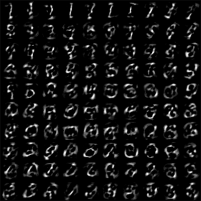
The above tiles are the images represented by each one-hot encoded vector (e.g. [0,0,….,X,….0]), and are useful to visualize the kind of forms the network is learning. This illustrates the patterns detected at layer 1 of the autoencoder for the MNIST dataset.

Other than this new weight initialization and pretraining, I found the best results with what seems to be the most standard network layout:

1. Encoder - The first half of each layer
   1. Gaussian Noise Layer - Add a specific amount of noise. This component is only active during training.
   2. Encoding Synapse Layer - Specially initialized as discussed above.
   3. Encoding Bias Layer - Initialized to 0
   4. Rectified Linear Unit - Truncates negative values. This simple feature is very effective in modern NNs, providing the needed nonlinearity without saturation effects.
   5. Dropout Layer - Randomly sets a certain % of outputs to 0, to encourage redundancy and reduce generalization error. This component is only active during training
2. Decoder - Decodes the encoded form, output from the encoder
   1. Decoding Synapse Layer - Initialized to be the transpose of the encoder synapse layer
   2. Decoding Bias Layer - Initialized to 0
   3. Rectified Linear Unit - Again, truncates negative values.

The final part of the standard MNIST autoencoder exercise is to take the new features and train a categorization network. We demonstrate this in the notebook, with our network achieving an end accuracy of about 90%. This accuracy does not match peer results, and I am looking into this.

One interesting result I noticed was the effect of sparsity (as provided by the dropout layer) on the characteristic patterns learned by the first level of the autoencoder. Previously shown is the result without sparsity, and the resulting visualization with 10% dropout during training is by comparison uninteresting. In the first, the network seems to learn patterns that have many long-range dependencies; the characteristic patterns look like some unidentifiable language… maybe ancient Chinese or elvish? The network with 10% dropout seems to learn much local patterns, consisting of an isolated line here or a curve there. However, the classification results produced by using the resulting features proved far more useful for classification.

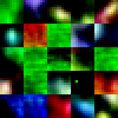
When this same procedure is run over a typical image, such as in this notebook, we produce some very different features:

As we venture deeper into the jungle of AI, it becomes clear we need certain tools. One of these tools is of course a computer interface, but when we do research, what interface should we use? Many patterns have emerged over the years, such as console, GUIs, web services, test cases, REPL, notebooks, etc. In AI computing we want to optimize for developer productivity and technical information, both of which make both the REPL and Notebook patterns attractive. This motivated a logging tool that makes it easy to produce markdown reports which quote code, providing a nice tool for static reporting based on pre-coded scripts.

Static reports, however, are chronically limited to run according to how it is coded to initially; there is no interactivity, and the output is strictly linear. Using a very similar interface, though, a lightweight interactive service can be set up to serve HTTP requests from a random port. This server provides common functions such as streaming logs, and can be extended for arbitrary interactivity. These two contexts, static and interactive, are united by a common logging interface for simple code reuse.

I hope you enjoyed this quick walk-through. Stay tuned for more!