Website request latencies, as a dataset, are odd. I can think of no other dataset I have encountered so frequently in my work, but when you do research about this dataset online, you find amazingly little compared to similar topics. Therefore, let’s talk about this today - specifically, what does the ideal statistical model for website latency look like?

The background for statistical modeling is large, and it is covered in several different approaches. I prefer intuitive arguments and an information-theoretic approach, so for background I refer readers to these articles:

• https://en.wikipedia.org/wiki/Information_theory
• https://en.wikipedia.org/wiki/Cross_entropy
• https://en.wikipedia.org/wiki/Principle_of_maximum_entropy
• https://en.wikipedia.org/wiki/Maximum_entropy_probability_distribution

For an illustrative example of a probability modeling for timing events, let’s talk about the Erlang distribution for a moment.

The Erlang Distribution

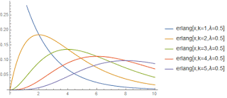
If we study the statistics of a timed event, we can first point out that the maximum entropy distribution of a positive variable with a given expectation value is the exponential distribution. If all we know is that the process latency can’t be negative, and we measure its mean value, this distribution is a natural choice.

However, if we look at many datasets, the latency is not only strictly positive, but it also trends quickly to zero near zero. That is, many processes cannot complete instantaneously and are unlikely to complete as fast as theoretically possible. One way to express this expectation could be that P[0]=0, P’[0]=0, P’'[0]=0 etc.

What if, just for fun, we modeled the time it would take for 2, 3, or more successive identical exponentially-modeled processes? That gives us a model with only one additional integer (“k”) parameter on top of the exponential’s single continuous parameter. The distribution is obtained via convolution operations, which produce what is known as the Erlang distribution. If we plot the first few values of k, we notice the behavior we sought above; each successive convolution has an additional 0 at a higher order derivative at x=0. It is obvious why k is called the “shape” parameter.

Our Dataset

In order to give our comparison a solid basis in reality, we use a publicly available dataset. I was surprised that I couldn’t find any publicly available access-log type datasets that include latency. I did, however, find the “King” dataset collected by and published by MIT. King is a tool to map out network latency based on multi-hop pings, so the dataset is essentially a radar map of the topology of the internet. We only use a very small slice of a small chunk of this dataset - 100k records of ping times across a single network link.

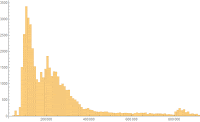
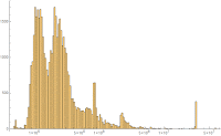
This dataset has several noticeable characteristics. First, it has a minimum time that is measurably positive - website requests never complete instantly or, of course, faster! Second, it has a really long tail. Both of these facts suggest we should look at the data in the Log[x] domain, which shows a few additional features. First, it appears to have a pair of Gaussian peaks, and a third broad-spectrum Gaussian curve. These curve shapes in the Log[x] domain suggest a Log-Normal model. However, the graphs suggest additional artifacts such as spikes and even-longer-tail behavior.

Models Considered

For this analysis we discuss several different models. Models consist of the following distribution families:

• Hypoexponential Distribution (e.g. Erlang Distribution) - Models successive exponential processes. The general case allows events to have varying expectations, Erlang models assume them to be identical.
• Gamma Distribution - An alternate generalization of the Erlang distribution, where the “number” of identical successive events modeled may be non-integer. (e.g. shape parameter of k=1.3)
• LogNormal Distribution - A Gaussian distribution remapped via e^x
• Pareto Distribution - This distribution is useful in modeling a number of phenomena exhibiting power-law long-tail behaviors. It is essentially a Log remapping of an exponential distribution.
• Mixture Models - Sub-models can be combined in a linear combination to produce a mixed model. Note there are many logical ways to combine two models, this being only one. Another would be convolution as we discussed with the Erlang distribution. Mixture models are mathematically convenient as they allow the Expectation-Maximization algorithm to be used.

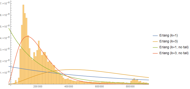
Additionally, it was found that long-tail effects severely distorted fitting the shape of the distribution in the “body” for several of the models used. To examine this effect, we also examine models fit against a filtered “no tail” dataset which excludes items over 500k.

A detailed walk-through of the process used to obtain each model is provided in the source Mathematica notebook.

Results

To summarize the results, I have grouped the models by the number of parameters used in the model.

1 Parameter Models

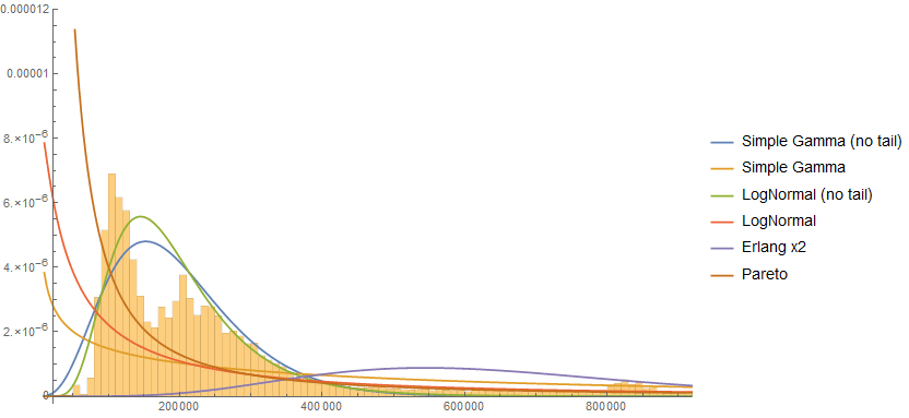
For 1-parameter models, I tested selected k values for the Erlang distribution. Shown are curves fit against the full dataset and curves fit on a truncated (non-tail) dataset.

2 Parameter Models

I tested six variants of 2-parameter models: Erlang (2-component mixture model), Gamma, Log-Normal, and Pareto (type II). Both the Gamma and Log-Normal distributions can fit the body shape but are distorted severely by tail effects, very similar to the single-variable Erlang curves.

4 Parameter Models

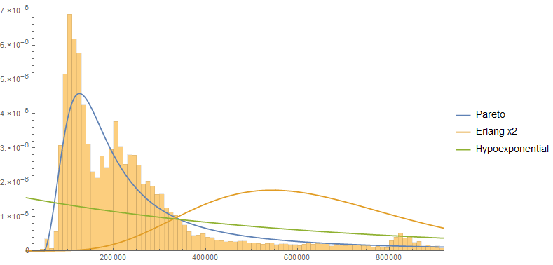
I tested three models with four parameters. Notably, the Pareto (type IV) model fits both the body and the tail quite well. I was also surprised that neither the hypoexponential nor Erlang mixture models converged on the body shape.

5+ Parameter Models

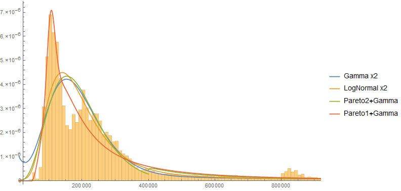
I also tested a variety of models that had 5 to 8 parameters. For details on the construction of these models, please refer to the source notebook. Different models fit different parts of the curve quite closely, and they seem to have similar performance determined mainly by the number of variables. This may not be entirely surprising if you consider they are all based on exponential distributions, but it is a notable result - the choice of distribution may matter less than how many variables you choose to allow in your model. All of these models were fit against the entire dataset, unfiltered and unbiased.

Conclusion

So what model wins? If I had to choose one, I’d say Pareto, but it depends on things like what you are using the model for and how you need to estimate it. If using a simple model such as Erlang, keep tail effects in mind. Another consideration is how to fit these models; moments, entropy, expectation-maximization, stochastic gradient descent… but that’s a topic for another day.

For details on these models, I’ve posted the Mathematica notebook in CDF format. There is a free reader available.